16. Hovmoeller Plot
16.1. Description
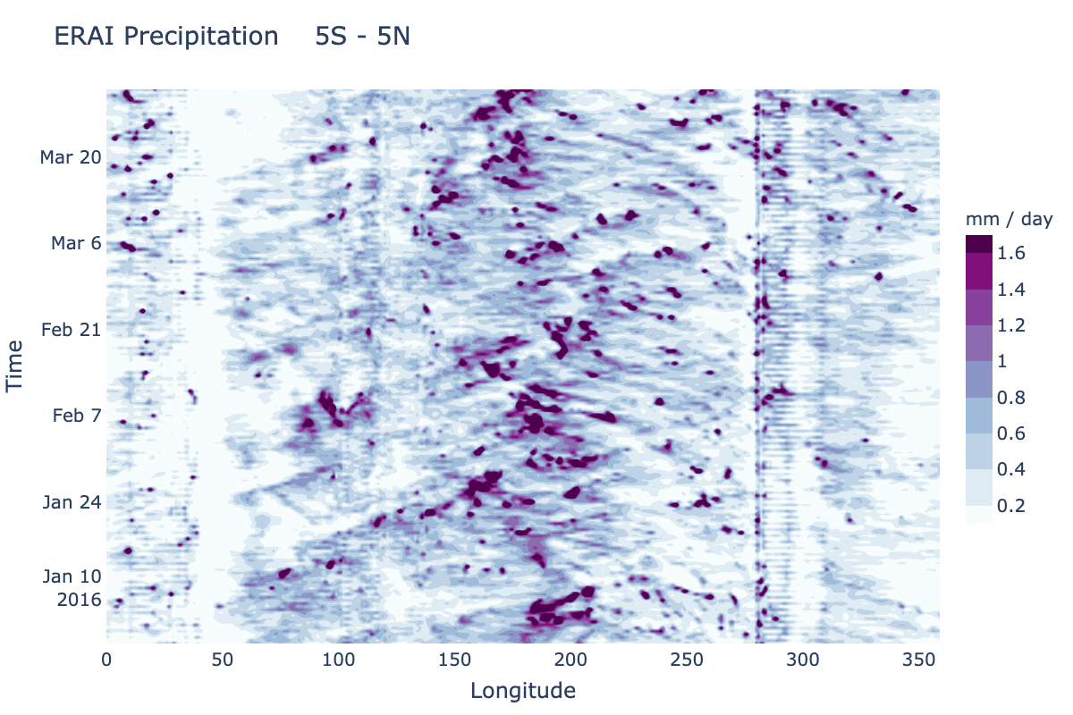
A Hovmoeller plot is a 2D contour plot with time along one axis and a spatial dimension along the other axis. Typically the spatial dimension not shown has been averaged over some domain. The current METplotpy Hovmoeller class supports only time along the vertical axis and longitude along the horizontal axis. This can be generalized in future releases to allow, for instance, time on the horizontal and latitude on the vertical. The examples are based on tropical diagnostics applications, so a meridional average of precipitation from 5 S to 5 N has been set up in the default configuration.
Please refer to the METplus use case documentation for instructions on how to generate a Hovmoeller diagram.
16.2. Required Packages:
metcalcpy
netcdf4 1.5.6
numpy 1.20.2
pandas 1.2.3
plotly 4.14.3
scipy 1.5.3
xarray 0.16.0
16.3. Example
16.3.1. Sample Data
The sample data used to create an example Hovmoeller plot is available in the s2s METplus data tar file in the directory model_applications/s2s/UserScript_obsPrecip_obsOnly_Hovmoeller.
Save this file in a directory where you have read and write permissions, such as $WORKING_DIR/data/hovmoeller, where $WORKING_DIR is the path to the directory where you will save input data.
16.3.2. Configuration Files
There is a YAML config file located in $METPLOTPY_BASE/metplotpy/plots/config/hovmoeller_defaults.yaml
plot_filename: erai_precip.png
height: 800
width: 1200
title: ERAI Precipitation

font_size: 20

xaxis_title: Longitude
yaxis_title: Time

date_start: 2016-01-01
date_end: 2016-03-31

lat_max: 5
lat_min: -5

var_name: precip
var_units: mm / day
unit_conversion: 250

contour_min: 0.2
contour_max: 1.6
contour_del: 0.2
colorscale: 'BuPu'
$METPLOTPY_BASE is the directory where the METplotpy code is saved:
e.g.
/usr/path/to/METplotpy if the source code was cloned or forked from the Github repository
or
/usr/path/to/METplotpy-x.y.z if the source code was downloaded as a zip or gzip’d tar file from the Release link of the Github repository. The x.y.z is the release number.
16.4. Run from the Command Line
To generate the example Hovmoeller plot (i.e. using settings in the hovmoeller_defaults.yaml configuration file) perform the following:
If using the conda environment, verify the conda environment is running and has has the required Python packages specified in the Required Packages section above.
Set the METPLOTPY_BASE environment variable to point to $METPLOTPY_BASE. where $METPLOTPY_BASE is the directory where you saved the METplotpy source code (e.g. /home/someuser/METplotpy).
For the ksh environment:
export METPLOTPY_BASE=$METPLOTPY_BASE
For the csh environment:
setenv METPLOTPY_BASE $METPLOTPY_BASERun the following on the command line:
python $METPLOTPY_BASE/metplotpy/plots/hovmoeller/hovmoeller.py --datadir $WORKING_DIR/data/hovmoeller --input precip.erai.sfc.1p0.2x.2014-2016.nc
where $METPLOTPY_BASE is the directory where you are storing the METplotpy source code and $WORKING_DIR is the directory where you have read and write permissions and where you are storing all your input data and where you copied the default config file. You will see informational output to the screen:
a usage statement
reminder to set the METPLOTPY_BASE:
“METPLOTPY_BASE needs to be set to your METplotpy directory”
logging information
A plot named erai_precip.png will be generated in the directory from which you ran the plotting command: